How does random tie-breaking during quantile normalization affect GWAS?

• By: Faith Okamoto
• Original analysis: early 2023
• Writeup: July 2024

Introduction

Palmer Lab performs genome-wide association studies (GWAS) on phenotypes meant to model complex human traits such as addiction. Many of these traits are non-normally distributed. For example, "number of lever presses" may measure desire for a drug, but is usually discrete and 0-inflated. Therefore, we use rank-based inverse quantile normalization (Bliss et al. 1956) before GWAS. This creates traits following the standard normal distribution. While such normalization is standard practice, it has some pitfalls, especially when many ties are present in the raw values (e.g. see Beasley et al. 2009).

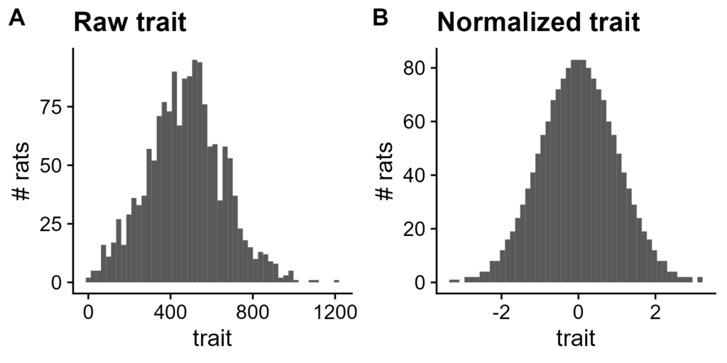
_{Figure 1. Example of quantile normalization on a somewhat normal trait. Histograms (with 50 bins) pre- and post-normalization of d1_magazine_ncs, i.e. number of intertrial interval magazine entries on day 1 of testing. A. Pre-normalization B. Post-normalization.}

Ties are a problem for rank-based normalization. All samples must be assigned distinct ranks. Therefore, all ties must be broken in some way. Tie-breaking methods include the order samples appear, the alphanumerical order of sample identifiers, or randomly by a pre-determined seed number. We seek to determine the extent to which particular tie-break choices affect the GWAS results.

Materials & Methods

Dataset

All data were taken from "Identification of Neurochemical Antecedents and Consequences of Distinct Learning Processes Relevant to Addiction Liability", Dr. Shelly Flagel's grant R21DA045146 (internal database name: pavca_MI).

3,513,494 autosomal single nucleotide polymorphisms (SNPs) in 6,147 rats were called by our standard genotyping pipeline (Chen et al. 2023) on reference genome Rnor_6.0, and archived. SNPs were filtered by standard thresholds:

• minor allele frequency (MAF) of ≥ 0.005
• missing rate of ≤ 0.1
• Hardy-Weinberg equilibrium p-value of ≥ 10^-10

3,507,340 remained and were used in association analyses. Then, 1,583 rats were subset as having useful phenotypes.

The original GWAS report (summary of results) is available.

Traits chosen

Three different traits, each with at least one significant quantitative trait locus (QTL) in the original analysis, were chosen. Each has a different kind of skew. All traits have many ties.

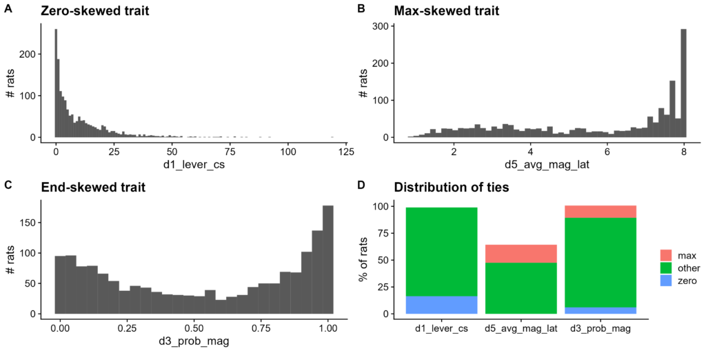
_{Figure 2. Distribution of non-normal traits chosen for study. A-C. Histograms of trait raw values. A. d1_lever_cs, a zero-skewed trait. Bin width of 1. B. d5_avg_mag_lat, a right-skewed trait. 50 bins. C. d3_prob_mag, an end-skewed trait. Bin width of 0.04. D. Number of values within a tie for each trait. Ties split into three categories: zero, max (tied with the maximum value), and other.}

• Zero-skewed: d1_lever_cs, average lever contact number on day 1 of testing. This is often 0, as many rats do not contact the lever at all. Also, it is constrained to nonnegative integers
• Max-skewed: d5_avg_mag_lat, average magazine entry latency on day 5 of testing. This is often at its maximum value, as many rats do not enter during the entire 8-minute session, so their latency defaults to 8.
• End-skewed: d3_prob_mag, average magazine entry latency on day 3 of testing. This is often at extreme values, as many rats have by this point either decided to quickly enter or to not enter at all. Also, it is constrained to multiples of 0.04 between 0 and 1 inclusive.

Normalization method

Traits were normalized by a rank-based inverse quantile normalization, performed separately for each sex. That is, the following steps were done, first for males and then for females:

1. Rank all values. Break ties by order in which values appear in the data frame (i.e. for two identical values, assign the earlier one a smaller rank).
2. Generate the corresponding quantiles on the standard normal distribution.
3. Replace ranks with their quantiles.

The precise code may be summarized as follows:

# quantile normalize in place
qnorm_non_na <- function(x) {
  non_na <- !is.na(x)
  # generate an even spacing of cumulative densities (small to large)
  cds <- (1:sum(non_na)-0.5) / sum(non_na)
  # match up points from small to large with the normal distribution
  x[non_na] <- qnorm(cds)[order(order(x[non_na]))]
  return(x)
}

Five different normalizations were performed for each trait. Order was randomized each time. None of these traits had covariates regressed out during the original analysis. Thus, no covariate adjustment was performed here.

Calling QTLs

15 GWAS were conducted, for five versions of the three traits. GWAS were run using mixed linear model based association (MLMA) analysis and the leaving one chromosome out method (Yang et al. 2014). An autosomal genetic relationship matrix (GRM), including all SNPs except those on the current chromosome, was used to adjust for relatedness (Yang et al. 2010).

The threshold for calling a quantitative trait locus (QTL) was a -log10 p-value of 5.6 for the "top" SNP, as well as a supporting SNP within 0.5Mbp and 2 -log10 p-value points. If multiple such "top" SNPs existed on a chromosome, an iterative process was used to separate distinct QTLs. SNPs within 1Mbp, or with an r² of at least 0.4 and within 1,000,000 SNPs/11Mbp, were assumed to be part of the same QTL and thus were removed from consideration. This process repeated until no more significant SNPs remained.

Notably, no attempt at conditional analysis (using a top SNP as a covariate) was attempted.

Software

• GCTA version 1.26.0, used for running MLMA and calculating SNP heritability
• PLINK version 1.90p 64-bit (2 Jun 2015), used for LD calculations and general genotype filtration
• R version 4.2.3, used for plotting results. Packages used:
  • cowplot version 1.1.1, used for plot themes/arrangement
  • data.table version 1.14.8, used for data management
  • ggmanh version 1.2.0, used for Manhattan plots
  • ggplot2 version 3.5.1, used for general plotting

Some relevant code/data is in DropBox (Palmer Lab only); this was not put in GitHub as its data files are too big for comfort.

Results/Discussion

Different tie-breaks do not change SNP heritability

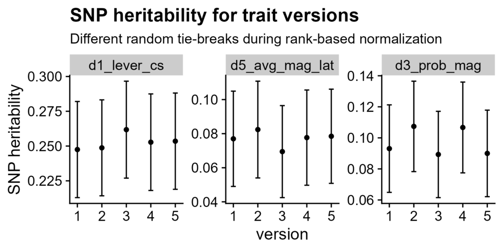
_{Figure 3. SNP heritabilities for different tie-break orders. Random tie-break versions grouped by trait. Error bars are +/- standard error.}

SNP heritability is the variance of a phenotype explained by considering all (autosomal) SNPs together, not just those which pass the QTL significance threshold (Yang et al. 2010). Different random tie-break orders do not affect this significantly; heritability is still within standard error.

Different tie-breaks change GWAS p-values

_{Figure 4. Example subtracted Manhattan plot. X-axis is position of SNP, split by chromosome. Y-axis is absolute value of difference between -log10 p-value for GWAS of Version 1 and Version 4 of d1_lever_cs. Points colored by whether they pass the significance threshold (-log10 p-value of 5.6) in one or both GWAs. All plots (one for each pair of versions of each trait) are available in DropBox (Palmer Lab only).}

Many SNPs dropped in and out of significance depending on tie-breaking. Some p-values, especially around QTLs, changed by large amounts.

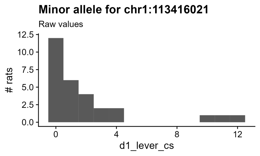
_{Figure 5. Raw values for rats carrying a minor allele at disputed QTL. X-axis is raw value of d1_lever_cs (bin width of 1). SNP is chr1:113416021. For distribution of all rats, see Figure 2A.}

For an example, see circled SNPs on Chromosome 1 with a change of over 2 -log10 p-value points. This QTL's SNP chr1:113416021 is heterozygous in 29 rats (no homozygous minor genotypes), for a MAF of 0.009. Similar to the distribution of this trait in general, these rats demonstrate a marked skew towards 0.

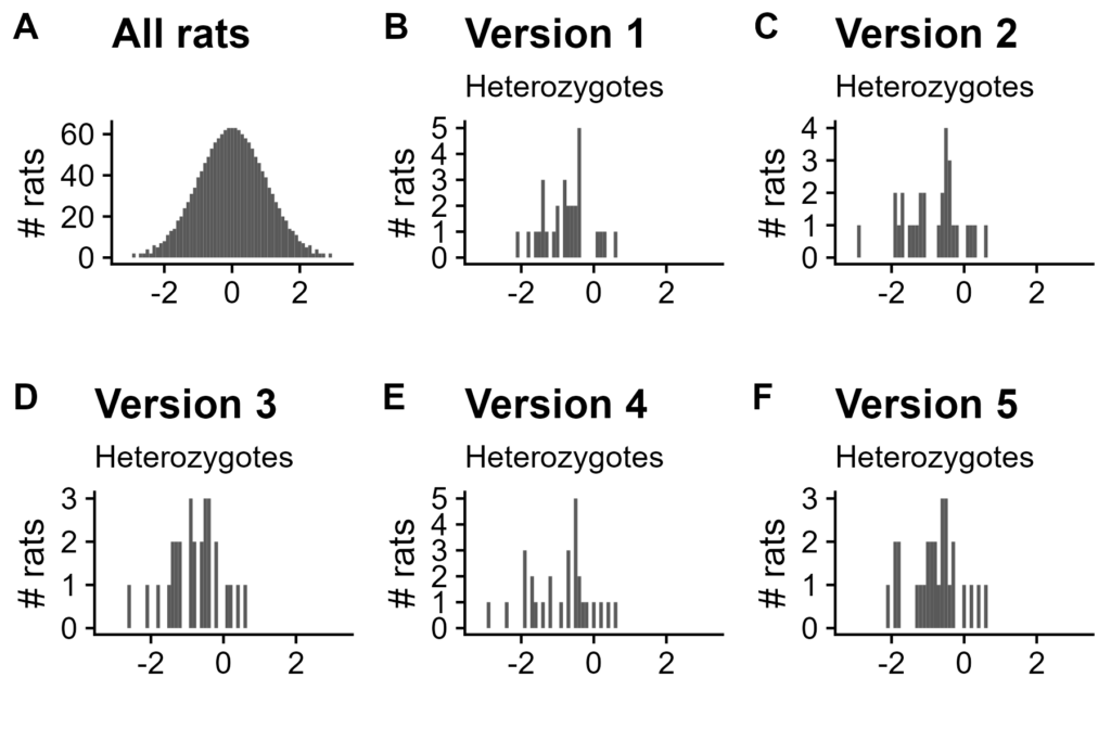
_{Figure 6. Normalized values for rats carrying a minor allele at disputed QTL. X-axis is quantile normalized value of d1_lever_cs (bin width of 0.1). A. All rats for Version 1. B-F. Rats with minor allele for each normalization version.}

Post normalization, however, their distribution varies wildly. This QTL was called in quantile normalization versions (i.e. random tie-breaks) 2, 4, and 5, but not in 1, 3, or the original analysis (Table 1).

Different tie-breaks change QTLs

For all traits considered in this article, QTLs were inconsistently called between different tie-break orders. Each QTL result is briefly discussed here. Again, see DropBox for all subtracted Manhattan plots.

d1_lever_cs

	Original	Version 1	Version 2	Version 3	Version 4	Version 5
chr1:113416021	No	No	Yes	No	Yes	Yes
chr5:56280155	Yes	Yes	Yes	Yes	Yes	No

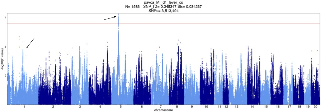
_{Figure 7. Original d1_lever_cs Manhattan plot with QTLs pointed out. X-axis is position of SNP, split by chromosome. Y-axis is -log10 p-value. Peaks which correspond to QTLs in any tie-break version are pointed to.}

Depending on how ties are broken, QTLs on two different chromosomes (1 and 5) may be present. The disputed QTL on Chromosome 1 was not picked up in the original analysis, and thus its possible importance was not considered.

d5_avg_mag_lat

	Original	Version 1	Version 2	Version 3	Version 4	Version 5
chr17:56513004	Yes	Yes	No	Yes	No	Yes

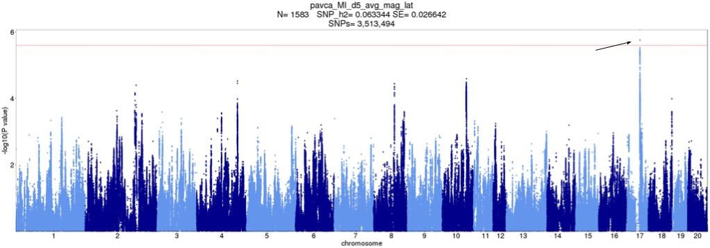
_{Figure 8. Original d5_avg_mag_lat Manhattan plot with QTLs pointed out. X-axis is position of SNP, split by chromosome. Y-axis is -log10 p-value. Peaks which correspond to QTLs in any tie-break version are pointed to.}

Depending on how ties are broken, the disputed QTL on Chromosome 17 (which was picked up in the original analysis) may be present; its SNPs drift in or out of significance. Notably, if tie-breaks like Version 2 or 4 were used for the original analysis, this trait would have been discarded as insignificant.

d3_prob_mag

	Original	Version 1	Version 2	Version 3	Version 4	Version 5
chr17:57301086	Yes	No	Yes	Yes	Yes	No
chr17:57442494	No	Yes	No	No	No	Yes

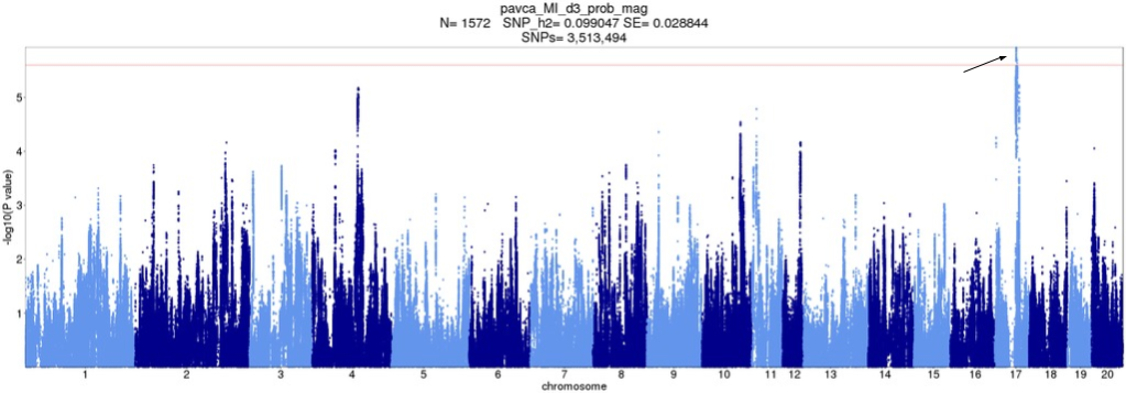
_{Figure 8. Original d3_prob_mag Manhattan plot with QTLs pointed out. X-axis is position of SNP, split by chromosome. Y-axis is -log10 p-value. Peaks which correspond to QTLs in any tie-break version are pointed to.}

Depending on how ties are broken, the QTL on Chromosome 17 shifts position slightly. Thus, the implicated/prioritized genes would have been different. Additionally, Version 5 had an extra QTL, at chr17:56436494 (1.006Mbp away, with an r² of 0.38). This is probably an artifact of the lack of conditional analysis.

Conclusion

There are alternative methods to deal with tied data, such as different normalizations (e.g., Peng et al. 2007) or statistical tests (Beasley et al. 2009), but for the sake of standardization, Palmer Lab is unlikely to adopt them. Thus, ties must be broken somehow.

In traits with many ties, the exact way in which they are broken can have a massive impact, moving QTLs or even creating new ones. The tie-breaking method should be clearly documented. It may be worth breaking ties in a few different ways and comparing the results, especially for massively tied traits.

References

_{Beasley TM, Erickson S, Allison DB. 2009. Rank-Based Inverse Normal Transformations are Increasingly Used, But are They Merited? Behav Genet. 39(5):580–595. doi:10.1007/s10519-009-9281-0.}

_{Bliss CI, Greenwood ML, White ES. 1956. A Rankit Analysis of Paired Comparisons for Measuring the Effect of Sprays on Flavor. Biometrics. 12(4):381–403. doi:10.2307/3001679.}

_{Chen D, Chitre A, Cheng R, Peng B, Polesskaya O, Palmer A. 2023. Palmer Lab Heterogeneous Stock Rats Genotyping Pipeline. doi:10.5281/zenodo.10002191.}

_{Peng B, Yu RK, DeHoff KL, Amos CI. 2007. Normalizing a large number of quantitative traits using empirical normal quantile transformation. BMC Proceedings. 1(1):S156. doi:10.1186/1753-6561-1-S1-S156.}

_{Yang J, Benyamin B, McEvoy BP, Gordon S, Henders AK, Nyholt DR, Madden PA, Heath AC, Martin NG, Montgomery GW, et al. 2010. Common SNPs explain a large proportion of the heritability for human height. Nat Genet. 42(7):565–569. doi:10.1038/ng.608.}

_{Yang J, Zaitlen NA, Goddard ME, Visscher PM, Price AL. 2014. Advantages and pitfalls in the application of mixed-model association methods. Nat Genet. 46(2):100–106. doi:10.1038/ng.2876.}