Detecting errors by using genotype kinships

• By: Faith Okamoto
• Analysis: mid-2023 to early 2024
• Writeup: August 2024

This writeup encompasses three projects undertaken at different points in time. All analyses have been redone with the most recent data when applicable.

Introduction

Palmer Lab has performed genotyping on many batches of heterogenous stock (HS) rats. Each DNA sample is tied to an RFID. Errors such as sample mix-ups (swapping DNA samples) or sample duplicates (using a DNA sample twice) disrupt the assignment of genotypes to RFIDs. Several quality control (QC) steps are done to ensure quality genotypes. However, each QC is done individually by sample, and thus cannot catch sample duplicates, whose defining feature is two rats with near-identical genotypes.

The HS rat population has a complicated breeding history, changing labs multiple times. While a pedigree exists, it is incomplete and likely has errors. Nevertheless it is mostly correct. This suggests a possible QC step: concordance between genetic and pedigree relatedness. For example, if a litter of six rats has intra-sibling first-degree genetic relatedness, except for one rat who appears unrelated, then that odd one out indicates an error in either the pedigree or the genotypes. If two rats were sequenced together and appear to have swapped litters, then they may be sample mix-ups.

Sample duplicate and pedigree mix-up QCs use genetic kinship. There is a base level of relatedness among all HS rats from shared genetic history: outbred from eight inbred strains (Hansen and Spuhler 1984), then maintained as an intrabreeding population. Put blithely, everyone is everyone's second cousin. Herein two methods to calculate genetic kinship are considered:

• Kinship-based INference for Genome-wide association studies (KING) "robust" coefficients (Manichaikul et al. 2010)
• GCTA-style genetic relationship matrix (GRM) off-diagonal values (Yang et al. 2010)

Then, sample duplicate and pedigree discordance QCs for HS rats are developed.

Materials & Methods

Dataset

The pedigree was collected from multiple sources. It was obtained internally from Riyan Cheng on 28 February 2024, then modified to drop records missing a sire/dam (10,929 rows), with a matching sire/dam (39 rows), and the two rats with a female rat listed as a sire. The final pedigree had sires and dams for 26,106 rats, with 26,720 unique RFIDs (including rats appearing only as parents).

HS rats were sequenced by ~0.25x coverage double-digest genotyping by sequencing (Gileta et al. 2020) or low-coverage whole-genome sequencing. Biallelic single nucleotide polymorphisms (SNPs) on mRatBN7.2 were imputed by STITCH as described in Chen et al. 2023. Full genotypes are archived.

Rats were filtered to only those which appeared in the pedigree (either as a child or a parent). SNPs were filtered by standard thresholds:

• minor allele frequency (MAF) of ≥ 0.005
• missing rate of ≤ 0.1
• Hardy-Weinberg equilibrium (HWE) p-value of ≥ 10^-10

The QC'ed dataset had 5,343,825 SNPs called in 15,230 rats, not pruned for linkage disequilibrium (LD), as is sometimes done when calculating kinship. The KING manual advises against such pruning, and Palmer Lab does not LD-prune the GRMs it uses for normal analyses.

Calculating kinship

Kinship was calculated in two ways:

• KING: --make-king triangle bin4 from PLINK 2.0. Duplicate samples/monozygotic twins have a KING kinship of 0.5.
• GRM: --make-grm-bin from PLINK 2.0. Duplicate samples/monozygotic twins have a GRM kinship of 1.

Input genotypes were filtered as in "Dataset".

Software

• PLINK version 2.00a5.12LM 64-bit Intel (25 Jun 2024)
• Python version 3.10.11, used for pedigree QC. Packages used:
  • pandas version 1.5.3, used for data management
  • base modules itertools, os, sys, and typing
• R version 4.2.3, used for data analysis. Packages used:
  • cowplot version 1.1.1, used for plot themes/arrangement
  • genio version 1.1.2, used for reading PLINK-binary files
  • ggplot2 version 3.5.1, used for general plotting

Code was deposited in GitHub for Palmer Lab members.

Results/Discussion

KING is superior to GRM to identify sample duplicates

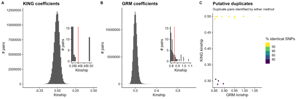
_{Figure 1. Testing sample duplicate identification. A-B. Histograms of kinship values. Kinship value on X-axis, count of pairs of rats on Y-axis. A. All KING kinships. Inset is zoomed in so the minimum X value is 0.35 and the maximum Y value is 15. Red line at 0.4 indicates chosen cutoff. B. All GRM kinships. Inset is zoomed in so the minimum X value is 0.8 and the maximum Y value is 15. Red line at 0.85 indicates chosen cutoff. C. Verifying sample duplicates from either method. GRM kinship on X-axis, KING kinship on Y-axis. Points colored by share of identical SNP genotypes.}

The simplest kinship QC is to find identical genotypes. Both KING and GRM kinships were tested for this purpose.

First, KING kinships. These cluster around 0. Zooming in, there is a clear gulf between high first-degree relatedness (e.g. siblings randomly sharing extra DNA) and duplicates. A cutoff of 0.4 worked well to separate duplicates, even though higher than the standard 0.354 (personal communication with Wei-Min Chen, Manichaikul et al. 2010 corresponding author). By this definition, there are 11 pairs of duplicate samples (22 unique samples).

Next, GRM kinships. These also cluster around 0, reaching around 1. Zooming in does not reveal a clear gulf. However, since all KING duplicate pairs had GRM values greater than 0.85 (minimum 0.853), that was chosen as a cutoff. By this definition, there are 15 pairs of duplicate samples; the 11 pairs from KING, and four more pairs with 7 more unique samples. The sample within two pairs is quite suspicious. Its putative duplicates should be putative duplicates of each other.

Finally, which kinship method produced better putative sample duplicates? All of the KING pairs have an extremely high share of identical raw genotypes, but the four pairs added by GRM kinships are less identical. This indicates the KING duplicates are reliable, but some GRM duplicates are not. No GRM cutoff can be used without either missing duplicates or implicating non-duplicates.

From this point on, only the more reliable KING kinships are used.

Development of sample duplicate QC

A simple sample-duplicate QC has two basic steps:

1. Calculate KING kinships between all pairs of rats, writing any pairs with kinship at least 0.4 to a file.
2. Create a file with two columns: RFID (IID in PLINK), and pass/fail. The latter is determined by whether the RFID appears in the file from step 1.

Assuming $GENO has been set to a --bfile prefix, and $OUT has been set to an output file prefix:

plink2 --bfile $GENO --make-king-table --out $OUT \
    --geno 0.1 --maf 0.005 --hwe 1e-10 --keep $OUT.temp.qc_ids \
    --king-table-filter $MAX_KING --chr 1-20

# determine QC result for all IDs, based on membership in failed IDs
cut -f 2 $OUT.temp.qc_ids | sort > $OUT.temp.rfids
cut -f 2,4 $OUT.kin0 | tail -n +2 | tr "\t" "\n" | sort \
	awk -F "\t" '{print $1, "fail"}' > $OUT.temp.fails
join -a 1 -j 1 -e pass -o auto $OUT.temp.rfids $OUT.temp.fails | tr " " "," > $OUT.csv

This was wrapped in a command-line script which also cleans up some of the intermediate files. On the most recent batch of HS rat genotypes (i.e. without being filtered by appearance in the pedigree), it takes around 3 hours with 5 cores when run on Palmer Lab's TSCC home node, with essentially the entire runtime being step 1 (first command in above code block). It identifies the 11 pairs of suspicious samples already noted in the last section, as well as one more pair including a rat missing pedigree data.

Identification of genotype-pedigree discordance

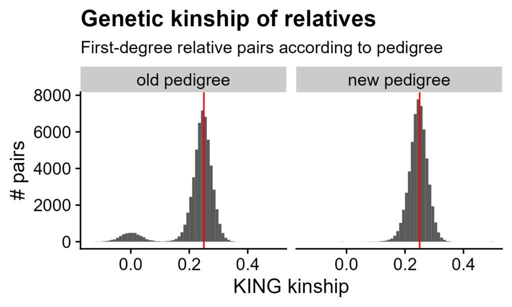
_{Figure 2. Genetic relatedness between pedigree relatives. Only siblings and parent/child pairs (i.e. first-degree relatives), according to the pedigree, are shown. Histograms of KING kinship coefficients: kinship on X-axis, count of pairs on Y-axis. Bins are multiples of 0.01. Red line is 0.25, the expected kinship between first-degree relatives. Left side is according to the original pedigree, right side is after family re-assignments.}

The initial pedigree, after removal of obvious issues (see "Dataset"), claimed that 55,804 pairs of genotyped rats were first-degree relatives. KING kinship coefficients have a main cluster around 0.25, as expected for first-degree relatives. However, there is a second cluster around 0, where unrelated HS rat pairs are (Figure 1A). Some pedigree relatives appear to actually be unrelated.

A Juypter Notebook identifies rats with discordant genotypes and pedigree assignment. First-degree relatives were used (mostly siblings as many parents were not genotyped). Genetic relatives were defined as a kinship of at least 0.18, which is the standard 0.177 rounded up.

1. Remove from consideration any rats with no genetic first-degree relatives. These can't be confidently assigned to anywhere.
2. Identify rats with discordant family assignments. This means that, of their genotyped first-degree pedigree relatives, less than 50% appear to be genetically first-degree relatives. Imagine a rat R with 5 littermates, where all of R's littermates are related to each other but not to R. This indicates R is in the wrong family.
3. Remove these rats from their families. For example, assign NA for R's family.
4. For each of those rats, identify the best family assignment. That is, the optimal pedigree family to maximize kinship to first-degree relatives. For example, another litter L consists of rats who all have first-degree relatedness with R. R will thus be assigned to have the same parents as L.
5. If step 4 resulted in changes in family assignments, the algorithm has not yet converged on the optimal pedigree. Thus, repeat steps 2-4.

After this, first-degree relatives have the expected kinships. 30 rats still could not be placed with concordant families. 87 other rats have no genetic relatives (i.e. were removed in step 1), of which 52 have no genotyped pedigree relatives (e.g. three-rat litter with two littermates taken as breeders).

Some sample duplicates changed litter assignments. Of the 11 duplicates pairs, two were already (and remained in) the same litter, one started in different litters and then both moved to the same new litter, and the rest had one rat be re-assigned to the other's litter. Rats whose "pair" moved to that rat's litter are likely the original, while the other is the duplicate.

Conclusion

Genetic kinship is a powerful tool to identify both sample duplicates and possible errors in the pedigree. KING-robust kinship coefficients, as implemented in PLINK 2, are well-suited for this. A few (12) pairs of genetically identical samples are present in the latest batch of genotypes.

There are many errors when comparing the pedigree to genetic kinships. However, as the pedigree is known to be faulty, none of these can be confidently determined as sample mix-ups.

References

_{Chen D, Chitre A, Cheng R, Peng B, Polesskaya O, Palmer A. 2023. Palmer Lab Heterogeneous Stock Rats Genotyping Pipeline. doi:10.5281/zenodo.10002191.}

_{Gileta AF, Gao J, Chitre AS, Bimschleger HV, St. Pierre CL, Gopalakrishnan S, Palmer AA. 2020. Adapting Genotyping-by-Sequencing and Variant Calling for Heterogeneous Stock Rats. G3 Genes|Genomes|Genetics. 10(7):2195–2205. doi:10.1534/g3.120.401325.}

_{Hansen C, Spuhler K. 1984. Development of the National Institutes of Health Genetically Heterogeneous Rat Stock. Alcohol: Clinical and Experimental Research. 8(5):477–479. doi:10.1111/j.1530-0277.1984.tb05706.x.}

_{Manichaikul A, Mychaleckyj JC, Rich SS, Daly K, Sale M, Chen W-M. 2010. Robust relationship inference in genome-wide association studies. Bioinformatics. 26(22):2867–2873. doi:10.1093/bioinformatics/btq559.}

_{Yang J, Benyamin B, McEvoy BP, Gordon S, Henders AK, Nyholt DR, Madden PA, Heath AC, Martin NG, Montgomery GW, et al. 2010. Common SNPs explain a large proportion of the heritability for human height. Nat Genet. 42(7):565–569. doi:10.1038/ng.608.}