Should GWAS in HS rats use PCs as covariates?
- By: Faith Okamoto
- Original analysis: late 2022 & early 2023
- Writeup: July 2024
Apologies for the poor figure quality; they have not been remade. I've also managed to lose a lot of the intermediate files, so I don't know e.g. how many SNPs were used, or what R package versions were used.
Introduction
Palmer Lab performs genome-wide association studies (GWAS) with the goal of identifying genetic variants influencing complex traits. Before GWAS we adjust raw data for various covariates such as sex, batch, age, etc. This avoids spurious correlations.
Our heterogenous stock (HS) rat genotypes are high-dimensional: each sample/rat has millions of datapoints, in the form of single nucleotide polymorphism (SNP) genotypes. Principal component analysis (PCA) is a method for dimensionality reduction. It collapses these millions of SNPs into axes which explain the dataset's variance. For example, if only a few versions of Chromosome 1 were present in the population, a principal component (PC) could aggregate data from many Chromosome 1 SNPs to separate samples along a Chromosome 1 axis.
Best practice in human GWAS is to include the top principal components (PCs) as covariates (Privé *et al. 2020). This corrects for population stratification (Price et al. 2006), which is endemic in human data. The HS rat population has a complex population structure due to limited breeding capacity. This is despite efforts to maintain a stable and diverse genetic background, aiming to avoid the loss or fixation of specific alleles.
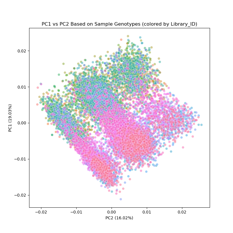
Figure 1. PCA biplot motivating this project. PC1 plotted vs. PC2 for 14,456 HS rats from a December 2022 run of the genotyping pipeline. Points colored by library preparation method (Riptide/low-coverage whole genome sequencing, vs. ddGBS/double-digest genotyping-by-sequencing).
This project evaluated the use of PCs as covariates in GWAS using HS rat data.
- Does using PC covariates have a significant effect on GWAS results?
- Does using PC covariates have a positive effect on GWAS results?
Materials & Methods
Dataset
All data were taken from the P50 center's Research Project 3, "Association between behavioral regulation and cocaine cue preference" (internal database name: p50_david_dietz_2020). SNPs were called by our standard genotyping pipeline on reference genome Rnor_6.0 (Chen et al. 2023). Raw phenotype data were pre-adjusted for all standard covariates.
In the interest of computational resources, only traits with significant results (using the original covariates) were re-analyzed.
Experimental GWAS covariates
GWAS were run using mixed linear model based association (MLMA) analysis, with a genetic relationship matrix used to correct for general relatedness (Yang et al. 2010), and the leaving-one-chromosome-out method (Yang et al. 2014). Two covariates were tested:
- Top 2 PCs. These were calculated using all genotypes in the study population.
- Project phase. Research Project 3 was a continuation of a previous project. A binary covariate encoded whether a rat was part of the previous project (as determined by an RFID starting with
000) or not.
As a control, GWAS were also run without either of these covariates. For these GWAS, only the original covariates were used. All GWAS used the same genetic relationship matrix with the leave one chromosome out method.
Software
- GCTA version
1.26.0, used for running PCA and MLMA - R version
3.6.1, used for plotting results. Also used were the packageschron,ggman,ggplot2, andggrepel
Results/Discussion
PC structure
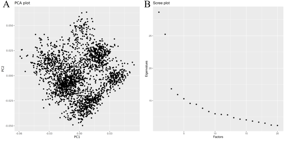
Figure 2. PCA on rats within Research Project 3. A. PCA biplot. PC1 on X-axis, PC2 on Y-axis. B. Scree plot for the top 20 PCs. Eigenvalue (relative variance explained) on Y-axis, PC number on X-axis.
The PC structure seen in Figure 1 is still visible even when sub-setting to only the rats within this project. Thus, this dataset is suitable for investigating the effects of using PCs. Second, as the scree plot shows, the first two PCs hold the most significance. After that, the amount of variance explained by each successive PC drops off quickly.
Based on these results, the first two PCs were used as covariates for the GWAS. Using too many PCs runs the risk of over-correcting the data.
Comparing GWAS
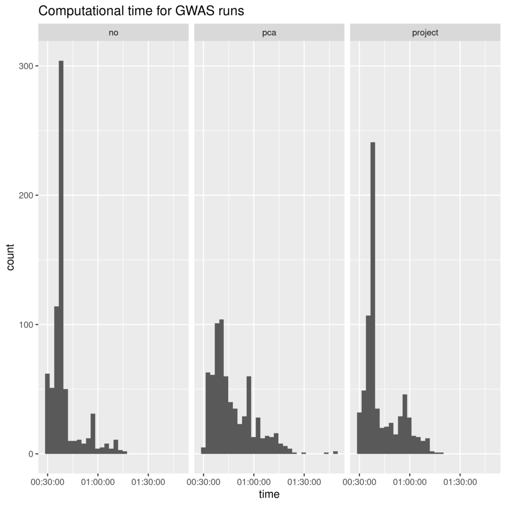
Figure 3. Time to run individual MLMA jobs. Histograms of time to run MLMA analysis for each chromosome-trait combination, split by which covariates were used: no additional ("no"), first two PCs ("pca"), rat from previous data vs. extension ("project").
Using PCs as covariates dramatically slows computation relative to the binary covariate (project) or no extra covariates. While there are high outliers, one main way this increase is achieved is a reduced clumping of short times. Perhaps PCA covariates prevented simplifications or easy optimizations which were available for the control and (to a lesser extent, "project") groups.
This was somewhat unexpected, as PC covariates can sometimes speed up human GWAS (Abraham Palmer, personal communication).
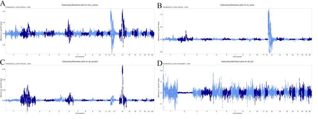
Figure 4. Subtracted Manhattan plots. X-axis is position of SNP, split by chromosome. Y-axis is difference between -log10(p) value for control GWAS and GWAS with additional covariate. Positive numbers indicate higher (i.e. more significant) -log10(p) values in the original GWAS. A-C. Representative subtracted Manhattan plots for PC covariates. D. Representative subtracted Manhattan plot for time/project covariates. All plots, including non-included ones, are available in Dropbox (Palmer Lab only).
A majority of the subtracted Manhattan plots for PC covariates have clear spikes around Chromosomes 13 and 14. Correcting for PCs made p-values less significant (especially when p-values were very significant, so there was further to fall). Correcting for time/project covariates produced much smaller and more uniform changes in p-values. However, it doesn't remove QTLs.
Conclusion
We decided that PC covariates didn't have positive effect to make up for the increase in computational time. Thus, they were not included in our standard GWAS pipeline.
References
Chen D, Chitre A, Cheng R, Peng B, Polesskaya O, Palmer A. 2023. Palmer Lab Heterogeneous Stock Rats Genotyping Pipeline. doi:10.5281/zenodo.10002191.
Price AL, Patterson NJ, Plenge RM, Weinblatt ME, Shadick NA, Reich D. 2006. Principal components analysis corrects for stratification in genome-wide association studies. Nat Genet. 38(8):904–909. doi:10.1038/ng1847.
Privé F, Luu K, Blum MGB, McGrath JJ, Vilhjálmsson BJ. 2020. Efficient toolkit implementing best practices for principal component analysis of population genetic data. Bioinformatics. 36(16):4449–4457. doi:10.1093/bioinformatics/btaa520.
Yang J, Benyamin B, McEvoy BP, Gordon S, Henders AK, Nyholt DR, Madden PA, Heath AC, Martin NG, Montgomery GW, et al. 2010. Common SNPs explain a large proportion of the heritability for human height. Nat Genet. 42(7):565–569. doi:10.1038/ng.608.
Yang J, Zaitlen NA, Goddard ME, Visscher PM, Price AL. 2014. Advantages and pitfalls in the application of mixed-model association methods. Nat Genet. 46(2):100–106. doi:10.1038/ng.2876.

Comments are closed.